Back to homepage Published July 6th 2026.

Kolmogorov complexity, Weight Entropy, Epiplexity

Dmitry Rybin

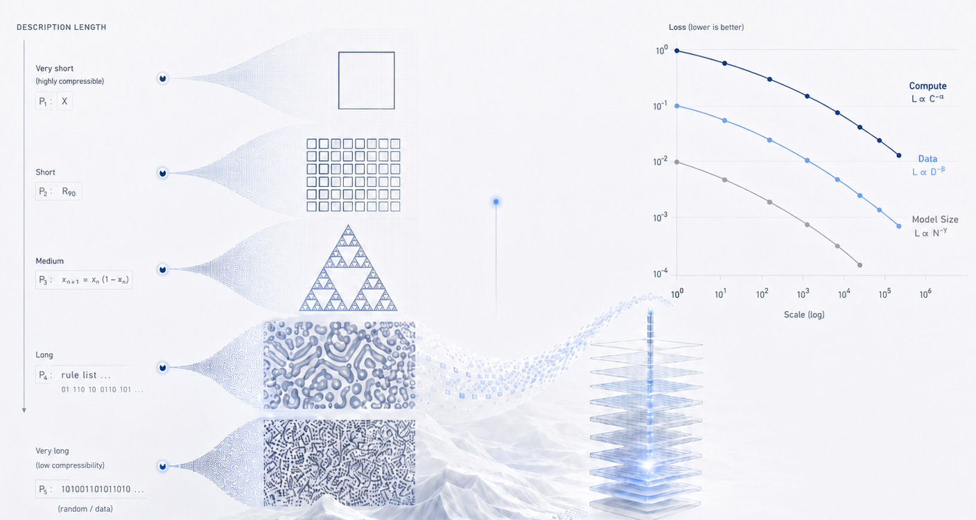
Kolmogorov complexity illustration

We go on an adventure connecting compute budgets, natural language structure, LLM scaling laws, Kolmogorov complexity of neural networks, theoretical importance of weight regularization, and epiplexity estimation. We derive generalization scaling laws and show that neural nets generalize as soon as the data is generated by processes of "moderate" Kolmogorov complexity.

Train and Test Loss

Our first goal is to find a connection between neural network loss on training data and test data. Assume that \(P\) is the probability distribution of the data and \(\mathcal{D}\) is a random sample from \(P\). If \(f\) is the prediction function, then \(\mathbb{E}_{P}L(f)\) is the expected loss on the whole distribution, while \(\mathbb{E}_{\mathcal{D}} L(f)\) is the training loss. There is a classical theoretical PAC bound1, which states that with probability \(1 - \delta\) we have \[\mathbb{E}_{P}L(f) \leq \mathbb{E}_{\mathcal{D}}L(f) +\sqrt{\frac{K(f)\log 2 + \log 1/\delta}{2|\mathcal{D}|}},\] where \(K(f)\) is the prefix-free Kolmogorov complexity of the function \(f\), and loss function \(L\) takes values between 0 and 1.

Here is the intuition why such a bound should exist. If the sample \(\mathcal{D}\) is random and large, then with high probability we have one of the two cases:

  • Case 1: \(f\) doesn't fit the data \(\mathcal{D}\) well.
  • Case 2: \(f\) fits the data \(\mathcal{D}\) well. Then, by law of large numbers, it must perform well for all big random samples \(\mathcal{D}\).

In either of these cases, for any specific \(f\), we can write with high probability: \[\mathbb{E}_{P}L(f) \leq \mathbb{E}_{\mathcal{D}}L(f) +\sqrt{\frac{\mathrm{something}}{2|\mathcal{D}|}}.\] But to get a bound that holds for any \(f\)2, we need to take a union bound over all possible functions \(f\). The space of neural networks is very large and naive union bound will become too loose. To bypass this issue we take a union bound with weights \(2^{-K(f)}\)3, which makes \(K(f)\) appear in the final bound.

So far we have used no properties of the data and neural networks. The generalization bound with Kolmogorov complexity holds for absolutely any distributions and functions.

Data and Neural Networks

Let's derive, from first principles, what properties of functions and data imply good generalization bounds.

First, we clearly want some \(f\) to be able to fit the data \(\mathcal{D}\) well.

Condition 1: The function class has universal approximation properties.

Second, we want the Kolmogorov complexity of \(f\) to be small. Specifically, with the dataset of size \(|\mathcal{D}|\), we want to have a function of Kolmogorov complexity \(o(|\mathcal{D}|)\) that fits the data. This constrains the nature of the data. Many works relate this property of natural language to the scaling laws.

Condition 2: The data has a structure that allows both \(\mathbb{E}_{\mathcal{D}}L(f)\) and \(\sqrt{K(f)/|\mathcal{D}|}\) to go to zero as \(|\mathcal{D}| \to \infty\).

Finally, we want to be able to compute such approximators \(f\) that have low Kolmogorov complexity.

Condition 3: Low Kolmogorov complexity estimators should be discoverable.

Luckily for us, neural networks and next token prediction data happen to experimentally satisfy all of these conditions. Our next goal is to derive precise generalization bounds for LLMs.
Generalization bounds for Large Language Models

Let's interpret and specialize the Kolmogorov-PAC bound for Large Language Models.

  • \(\mathbb{E}_{P}L(f)\) is the expected next token prediction loss of the model on the entire human text distribution.
  • \(\mathbb{E}_{\mathcal{D}}L(f)\) is the pre-training loss. According to the scaling laws4, it can be modeled as \(L(N, D) = L_{\infty} + \left(\frac{D_0}{D}\right)^{\alpha} + \left(\frac{N_0}{N}\right)^{\beta}\), where \(L_{\infty}\) is the irreducible loss (natural language entropy), \(D\) is the number of (context, next token) pairs in the training data, and \(N\) is the number of parameters of the LLM.
  • \(K(f)\) is the Kolmogorov complexity of the trained LLM. We want to discuss it in more details.

Kolmogorov complexity of LLMs

Any neural network can be described by layer weights \(W_l\) and specifications (architecture, tokenizer, number formats). This gives an upper bound \(K(f) \leq \sum_{l} K(W_l) + O(1)\). There are two ways to bound \(K(W_l)\):

  • Assuming the weight \(w_{l, ij}\) is represented with \(b_{l, ij}\) bits, we get \(K(W_l) \leq \sum_{i,j} b_{l, ij}\).
  • Experimentally, \(w_{l, ij}\) follow nice probability distribution \(P_l\). This gives another form of the bound via entropy of the weights \(K(W_l) \leq |W_l|H(P_l) + O(1)\).

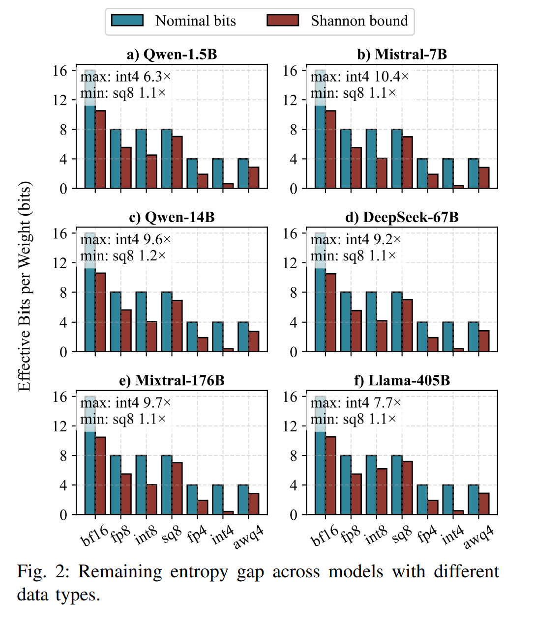
A recent work5 has computed weight entropy of several open models.

Weight entropy illustration

Using these bounds we get a simple generalization guarantee: \[ \mathbb{E}_{P}L(f) \leq L_{\infty} + \left(\frac{D_0}{D}\right)^{\alpha} + \left(\frac{N_0}{N}\right)^{\beta} + \sqrt{\frac{\sum_{l} |W_l|H(P_l) + O(1)}{D}}\]

This bound already reveals interesting heuristics. For a fixed dataset \(\mathcal{D}\) and a fixed achieved pre-training loss, the following quantities predict better generalization bounds:

  • lower precision of the weights,
  • lower \(L_1\) norm of the model weights,
  • lower entropy of the weight matrices \(W_l\).

Scaling laws for pre-training loss \(L(N, D)\) are used to predict the optimal neural network and dataset size for a given compute budget. Let's derive optimal allocation from generalization bound. Assume:

  • the compute budget is \(C \approx 6ND\) FLOPs,
  • the pre-training loss is \(L(N, D) = 1.8172 + 482.01 \cdot N^{-0.3478} + 2085.43 D^{-0.3658}\),
  • the Kolmogorov complexity is \(K(f) \approx cN^s\).

The objective function is \[\min_{C=6ND} 1.8172 + 482.01 \cdot N^{-0.3478} + 2085.43 D^{-0.3658}\ + \sqrt{\frac{cN^s \log 2 + O(1)}{2D}}\]

A short calculation for \(c=1\) and \(s=1\) reveals: \[ N^{*} = 34.07C^{0.3709} \qquad D^{*} = 0.00489C^{0.6290}\] For \(C=10^{26}\) FLOPs this gives \[N^{*} \approx 125B \qquad D^{*} \approx 130T\] In comparison, without the Kolmogorov complexity term, the prediction becomes \[N^{*} \approx 1.02T \qquad D^{*} \approx 16.4T\]

Epiplexity of LLMs

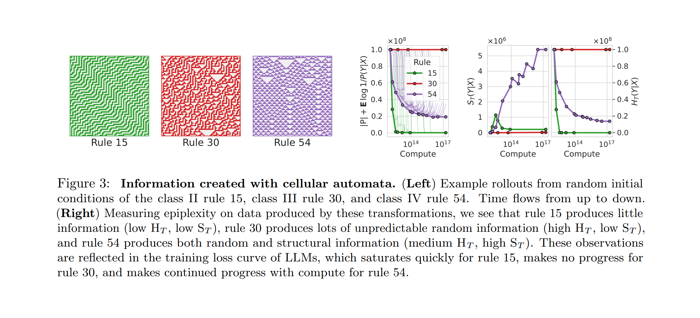
As a final note, we observe that our scaling laws predict that an LLM of Kolmogorov complexity \(K(f) \approx N \approx C^{0.3709}\) requires compute \(C = K(f)^{2.696}\) to be discovered (i.e. we spend \(K(f)^{2.696}\) on optimizing the neural network weights). Luckily, this is polynomial growth of compute. This is the great mystery of the compute-efficiency of modern NN training algorithms. A recent work has introduced epiplexity6 to quantify the amount of information that can be recovered from data under fixed compute budget.

Epiplexity illustration

References

  1. Anselm Blumer, Andrzej Ehrenfeucht, David Haussler, and Manfred K. Warmuth, Occam's Razor, Information Processing Letters, 1987.
  2. Sanae Lotfi et al., PAC-Bayes Compression Bounds So Tight That They Can Explain Generalization, arXiv, 2022.
  3. Tamay Besiroglu et al., Chinchilla Scaling: A replication attempt, arXiv, 2024.
  4. Justin Lovelace et al., Prescriptive Scaling Laws for Data Constrained Training, arXiv, 2026.
  5. Hongshi Tan et al., Approaching Shannon Bound with Lossless LLM Weight Compression, arXiv, 2026.
  6. Marc Finzi et al., From Entropy to Epiplexity: Rethinking Information for Computationally Bounded Intelligence, arXiv, 2026.

If you want to cite this note

@misc{Rybin2026LLMGeneralization,
  author = {Rybin, Dmitry},
  title = {Kolmogorov complexity, Weight Entropy, Epiplexity},
  year = {2026},
  howpublished = {\url{https://rybindmitry.github.io/blogs/why-llms-generalize-kolmogorov-complexity-weight-entropy-nns-epiplexity.html}},
  note = {Blog post}
}